In most projects, the data contains many repeated causal claims with the same cause and the same effect (often across many sources). We call these bundles (or co-terminal link bundles).

This extension is about:

• computing bundle-level statistics for repeated cause->effect claims, and
• being clear that links tables and maps display bundles differently.

Why bundling is useful (for practitioners)#

• Simpler maps: instead of 200 separate “A → B” rows, you see one “A → B” bundle with counts.
• Clearer evidence signals: you can read “how widely shared” (sources) vs “how often said” (citations).
• Better reporting: it’s easy to state things like “7 sources mentioned A → B”.

What you get#

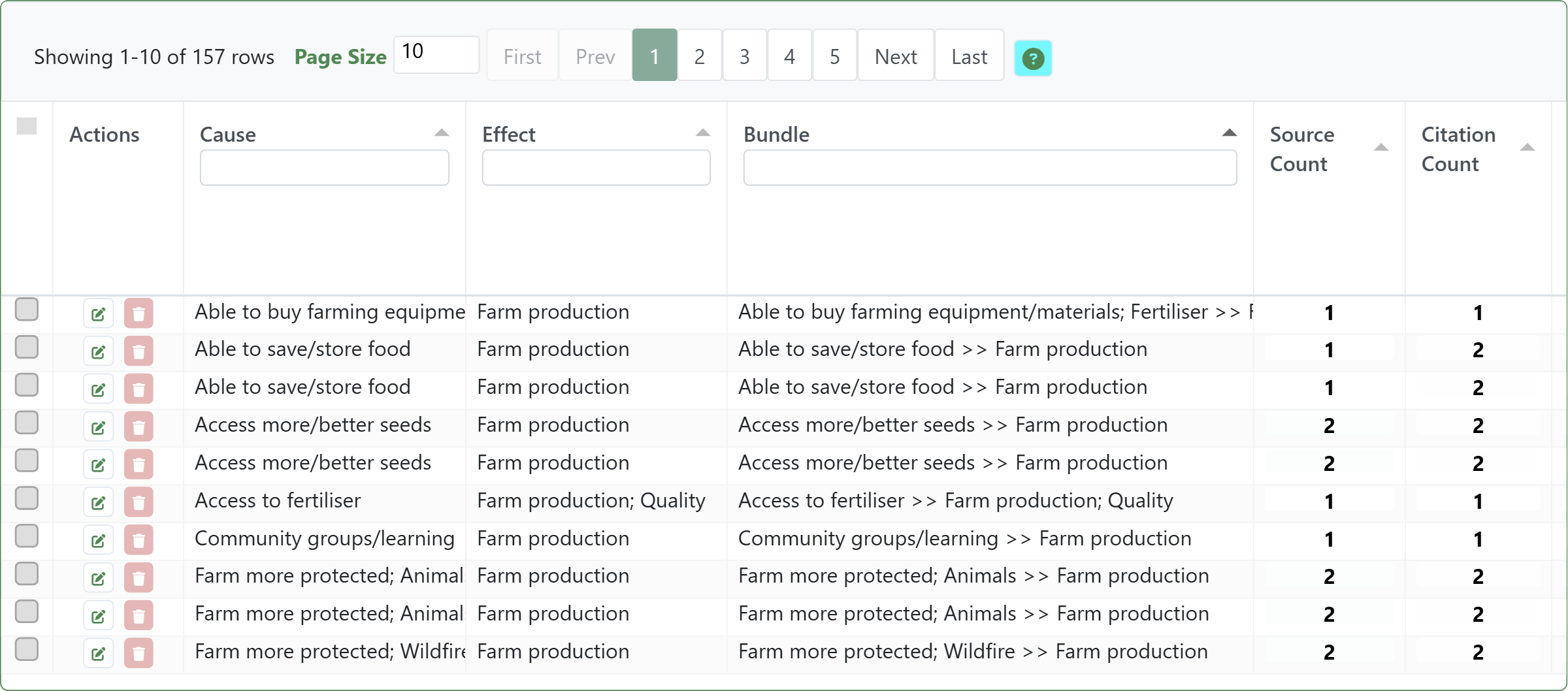
In the links table, each coded claim still appears as its own row (so you can still inspect individual claims/quotes separately).

What changes is that each row also gets bundle-level fields, computed from all rows with the same cause->effect pair (after transforms), for example:

• a readable bundle key like cause >> effect
• source_count (how many distinct sources made at least one claim of this form)
• citation_count (how many coded claims / rows are in the bundle)
• optional summaries like mean sentiment (if you use sentiment)

Rows in the same bundle share the same bundle-level values.

This means that however many filters you previously applied, including filters that might completely transform your factor labels, you still get exactly one row in the links table for every original causal claim which has not been filtered out by the filters.

Bookmark: #1143

How links are shown in tables vs maps#

• Links table: one row per coded claim/citation, with repeated bundle-level stats on each row in that bundle.
• Map view: one visual link per bundle (one unique cause->effect pair), not one per citation. This prevents an unreadable hairball.

So if a map link label says “7 sources / 12 citations”, read it as:

• 12 coded claims were bundled into that one displayed map link, coming from
• 7 distinct sources.

This map corresponds to the links table above.

![[008 Task 2 & 3 — Extensions/img/39412fad02d2b554610e8968d71a2d57_MD5.png|]]

Links — width: citation count; labels: source count. Filters applied: Labels: Farm production, match start. Bookmark #1144

Practical cautions#

• Bundling happens after transforms: if you zoom/collapse/combine opposites/cluster first, you are bundling the transformed labels, not the raw labels. That’s often what you want, but be deliberate.
• Counts are evidence volume, not effect size: a frequent bundle means “often claimed”, not “strong causal effect”.

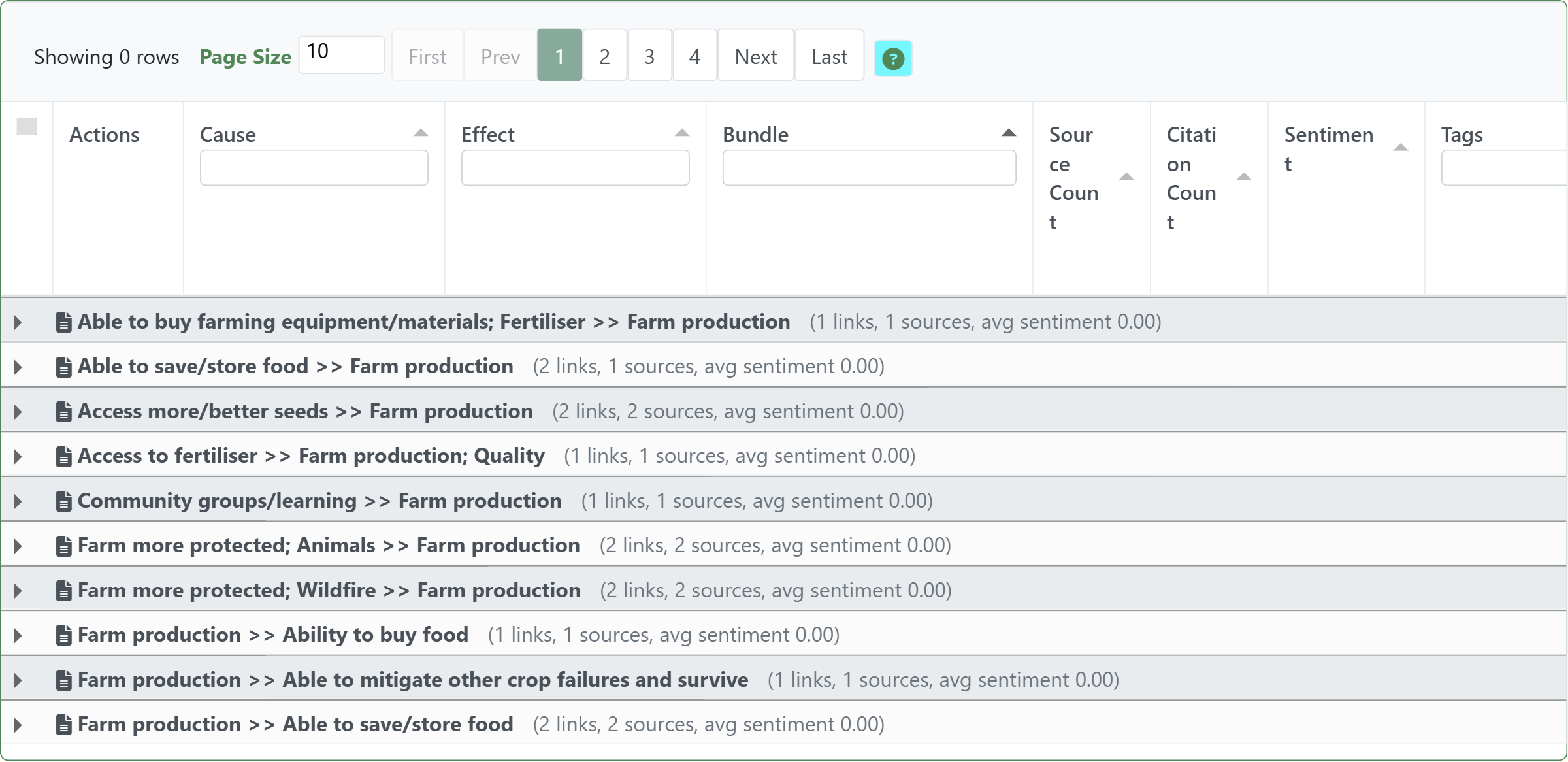
You can view the links table grouped into bundles#

In the Causal Map app, you can optionally group your links and factors and sources tables any way you want. In particular, you can group by bundle.

This view corresponds to bookmarks #1143 and #1144, above.

Formal notes (optional)#

The filter groups rows on the current (possibly transformed) labels using bundle key (cause label, effect label).

In links tables, grouped statistics are attached back to each underlying row. In maps, each group is rendered as one displayed link.

• Bundle key: (cause label, effect label)
• One bundle = one unique cause->effect pair

Bundle-level output fields include:

• bundle: a readable key like cause >> effect
• citation_count: number of underlying link rows in the bundle
• source_count: number of distinct sources contributing at least one link row to the bundle

Further summaries can be computed from the underlying rows (e.g. mean_sentiment, per-tag counts, per-group counts).

Other extensions like Opposites may themselves extend this extension. For example when combining opposite factor labels you may see additional columns in the links table.